
17 July 2026
Setting Up Object Tables in BigQuery to Analyse Unstructured Data
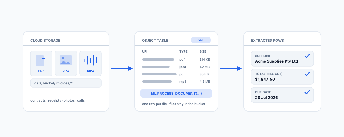
How to set up BigQuery object tables over Cloud Storage — the BigLake connection, the CREATE EXTERNAL TABLE step, and the ML functions that turn scanned invoices, contracts, images, and call recordings into queryable rows.
A data warehouse holds the tidy fraction of a business's data — the rows: sales, invoices, customers. Most of what a business actually accumulates is nothing like that. It is scanned receipts, signed contracts, product photos, call recordings, and PDFs of everything, sitting in folders and buckets where the only way to analyse them is to open them one at a time. BigQuery's object tables close that gap: they let the warehouse treat a Cloud Storage bucket full of files as a table you can query, and — combined with BigQuery's AI functions — turn the contents of those files into ordinary rows that sit alongside your structured data. Here is how to set one up, what analysing the content actually looks like, and where the costs and traps are.
What an Object Table Actually Is
An object table is a read-only, metadata-over-files table, powered by BigLake. Point it at a path in a Cloud Storage bucket and you get one row per file, with columns for the object's metadata — its URI, content type, size, and last-updated time. The files themselves never move: they stay in the bucket, and the object table is an index over them that SQL can see. That alone is useful — "how many contracts landed this month", "which product photos are older than the products they show" — but the real point is what it enables. Because the files are now addressable from inside BigQuery, they can be handed to AI functions for content analysis, with the results landing as structured rows. The warehouse stops being blind to everything that is not already a row.
What You Need Before You Start
The setup has four ingredients, and most of the friction lives in the second one:
- A Cloud Storage bucket holding the files, ideally organised under a clear prefix per document type — invoices/, contracts/, recordings/ — rather than one undifferentiated pile.
- A BigLake connection (a "Cloud resource" connection in BigQuery). This is BigQuery's bridge to Cloud Storage; creating it takes a minute in the console and produces a service account that belongs to the connection.
- Storage access for that service account — grant it the Storage Object Viewer role on the bucket. This is the step everyone forgets, and the symptom is a table that creates fine and then fails on query.
- A dataset in the same region as the bucket and the connection. Cross-region is the silent killer of first attempts; pick one region (for Australian data, typically australia-southeast1) and keep all three in it.
Setting the Table Up
With the ingredients in place, the table itself is a single statement: a CREATE EXTERNAL TABLE that names the connection and sets object_metadata = 'SIMPLE' plus the uris to index — for example gs://your-bucket/invoices/*. Run it and the object table appears in your dataset like any other table; selecting uri, content type, size, and updated over it lists your files as rows.
Two options in that statement deserve deliberate choices rather than defaults. The first is metadata caching (metadata_cache_mode and max_staleness): for buckets with many files, caching makes queries dramatically faster, at the price of results that can lag the bucket by the staleness window you set — an hour is a common, sane choice for business documents. The second is scope: index a specific prefix, not the whole bucket. A table over invoices/* has a clear meaning and a predictable size; a table over everything becomes an accidental catalogue of whatever anyone ever uploaded, and every downstream AI function you run over it inherits that mess.
Analysing the Content
The metadata table is the plumbing; the payoff is running BigQuery ML's remote-model functions over the files it indexes. Each follows the same pattern: create a remote model that points at a Google AI service, then call a function over the object table, and the extracted content comes back as rows.
- ML.PROCESS_DOCUMENT sends documents to Document AI. With one of the specialised processors, a folder of scanned invoices becomes a table of suppliers, ABNs, line items, totals, and due dates — the single most useful trick in this whole area for a small business.
- ML.ANNOTATE_IMAGE sends images to the Vision API: labels, detected text, and logos out of product photos or signage shots.
- ML.TRANSCRIBE turns audio files — call recordings, voicemails — into transcript text you can search and analyse.
- ML.GENERATE_TEXT with a Gemini model is the flexible one: prompt it against documents or images for anything the specialised processors do not cover, such as "summarise the termination clause in this contract".
Because the output is ordinary rows, the extracted data joins directly with everything else in the warehouse — invoice totals against your accounting feed, call transcripts against the deals they relate to. That joining is where the value compounds, and it is the same warehouse-first logic as our guide to getting CRM sales performance data into BigQuery. One newer development worth knowing exists: the ObjectRef data type (in preview) lets file references live as a column inside ordinary tables, rather than in a separate object table — the direction of travel is unstructured and structured data in the same row.
Access, Security, and Serving
Three details matter once real documents are involved. First, dashboards and apps that need to show the underlying file can use EXTERNAL_OBJECT_TRANSFORM to generate short-lived signed URLs from the object table, so Looker Studio can link to the actual invoice without the bucket being public. Second, row-level security works on object tables like any other table — the HR folder can exist in the same index as the invoices without being visible to the same analysts. Third, permissions are delegated through the connection: users query the table with BigQuery permissions alone and never need direct access to the bucket, which keeps the storage locked down to exactly one service account.
Costs and Gotchas
Object tables themselves are cheap; the surprises live around them:
- The AI functions are priced per call — Document AI, Vision, and Gemini each bill per document, image, or request. Running ML.PROCESS_DOCUMENT over ten years of archives without a WHERE clause is a real bill. Process incrementally — new files since the last run — and batch deliberately.
- Staleness versus refresh cost — aggressive cache refresh on a huge bucket costs money; a too-generous staleness window means this morning's files are missing from the table. Match the window to how often the analysis actually runs.
- Region mismatches fail late and confusingly. Bucket, connection, dataset, and remote models all in one region, always.
- Start with one folder and one question — "extract these fields from these invoices" — and expand once that works, rather than indexing the company's entire file history on day one.
What This Looks Like for a Small Business
Concretely, the setups we see earning their keep are modest ones:
- A receipts-and-invoices pipeline — supplier documents land in a bucket (often forwarded straight from email), ML.PROCESS_DOCUMENT extracts the fields, and a scheduled query reconciles them against the accounting feed.
- A contract register — one folder of signed agreements becomes a searchable table of parties, dates, renewal terms, and obligations, instead of a filing cabinet nobody opens until something goes wrong.
- A product image audit — ML.ANNOTATE_IMAGE over the catalogue's photos, joined to the product table, flags mismatches and missing images before customers find them.
- Call-recording review — transcripts of support or sales calls, searchable in SQL, with the interesting ones surfaced by a Gemini prompt rather than someone listening to hours of audio.
Getting Help
Object tables are one of those features where the setup is genuinely small — a connection, a permission grant, and one statement — but the design decisions around it (what to index, which processor to use, how to schedule and batch the extraction, and how to join the results into the rest of your data) decide whether it becomes a working pipeline or an expensive experiment. If you would like it scoped and built properly — from the Cloud Storage layout through the extraction models to the dashboards on top — our workflow automation service builds exactly this kind of pipeline end to end. Done once, properly, the pile of PDFs stops being a pile and becomes just another table.